
Chapter 16 covers how to find and download JSON and csv files and how to plot data from the files using Matplotlib and Plotly. We will be integrating what we learned about files in chapter 10 with what we learned about plotting data in chapter 15.
Examples from the chapter can be downloaded using the following link: Chapter_16.zip (this file includes data files you will need to complete the hands on exercises)
The csv examples in the lecture/demo, use the following file: foods.csv
For the assignment, you ONLY need to complete the hands-on exercises for your assignment (you don't need to complete all the small exercises within each chapter, although it is very good practice).
To see a video demonstration of the lecture material, watch: https://youtu.be/yT5ur2-i9aY
To see a video explanation of the hands on exercises, watch: https://youtu.be/sZQf1jTlxqg
A lot of data online can be downloaded as a csv (comma-separated value) file. Excel workbooks can export data in csv format and so can many database management systems.
Python has a module you can import that handles csv files
Syntax: import csv
The csv library contains objects and other code to read, write, and process data from and to CSV files.
The CSV file is opened as a text file and the file object is passed to a reader. Reading from a CSV file is done using a reader object or a dictonary object.
If you use a reader object, you can store the first row in a header variable. Each row of data retrieved is stored in a list.
Example reading the file, printing the first row and counting the rest:
Sample Output
['Food_Item_ID', 'foodcode', 'foodname', 'Protein (g)', 'Total Fat (g)', ' Carbohydrate (g)', ' Energy (kcal)']
['1', '11111000', 'Milk, whole', '3.1499', '3.25', '4.7999', '61']
Processed 6455 lines.
Example from the book reading the first row and storing it in a header_row variable
filename = 'data/sitka_weather_07-2018_simple.csv'
with open(filename) as f:
reader = csv.reader(f)
header_row = next(reader)
print(header_row)
Each example processes lines slightly differently. The first example processes the file line by line and the second uses a next() method.
When used in a loop, the next() method automatically returns the next item or line in a list until it reaches the end of file
Syntax: next(iterator)
Where the iterator is the file object
The function is useful when working with csv data because it lets you retrieve the index# and value. Since csv data typically comes from a spreadsheet, when you enumerate data in the first row, the index# is the column# and the data retrieved is the column heading.
Example:
Sample Output
['Food_Item_ID', 'foodcode', 'foodname', 'Protein (g)', 'Total Fat (g)', ' Carbohydrate (g)', ' Energy (kcal)']
0 Food_Item_ID
1 foodcode
2 foodname
3 Protein (g)
4 Total Fat (g)
5 Carbohydrate (g)
6 Energy (kcal)
['1', '11111000', 'Milk, whole', '3.1499', '3.25', '4.7999', '61']
Example from the book:
filename = 'data/sitka_weather_07-2018_simple.csv'
with open(filename) as f:
reader = csv.reader(f)
header_row = next(reader)
print(header_row)
for index, column_header in enumerate (header_row):
print(index, column_header)
If you use a dictionary object, the first line of data will be used to create keys (this line typicaly contains column headings from the spreadsheet). Each row of data is stored in a dictionary. In the sample output below, you will notice the number of items processed is one less than the list processing above BECAUSE the DictReader uses the first line as keys.
Example reading the file into a dictionary object,
Sample Output:
{'Food_Item_ID': '1', 'foodcode': '11111000', 'foodname': 'Milk, whole', 'Protein (g)': '3.1499', 'Total Fat (g)': '3.25', ' Carbohydrate (g)': '4.7999',
' Energy (kcal)': '61'}
{'Food_Item_ID': '2', 'foodcode': '11111100', 'foodname': 'Milk, whole, low-sodium', 'Protein (g)': '3.1', 'Total Fat (g)': '3.4599', ' Carbohydrate (g)': '4.4599', ' Energy (kcal)': '61'}
Processed 6454 lines.
To retrieve data, you can subscript into each row retreived using the index# (that is why it is useful to use enumerate to see the index# and values for each column)
If we wanted to retreive the name of the food, the protein, fat and carbs we would need to subscript into the list using index# 2,3,4 and 5. Once we retrieved the information, we could store it in our own dictionary or list.
Example:
NOTE: The data in the example has numbers or NULL values for protein, fats and carbs. I had to adjust the code to look for the NULL value and append a zero OR append the actual numeric value.
Python processes a large volume of data extremely fast. There are over 6000 entries in the foods.csv file and it processed them very quickly.
Once we have accessed the data and stored it in lists, we can chart the data using Matplotlib or Plotly.
When you are dealing with large data sets, you need to determine what type of chart will work best. Scatter plots work well for large volumes of data. The other chart types don't work quite as well.
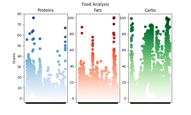
If you have too much data, you may need to create a subset to chart. The example below randomly retrieves data to chart because the protein, carbs and fat for over 6000 food items is too much for a single chart. If I wanted to see variance in protein, then I could chart 6000 foods and only look at protein
Example creating a subset of 500:
Sample Output
Example charting over 6000 proteins,fats and carbs in 3 separate scatter plots within 1 figure
Sample Output
1. Complete Try-It-Yourself 16-3. Name the file whatever you want. Feel free to change the type of chart to whatever you think looks good (if the line chart doesn't work for a temperature comparison, use something else)
NOTE: This is similar to the example in the book, BUT you will need to follow the instructions on pages 345-346 to download the San Francisco weather data (If you would prefer to chart a different city, that is OK as long as you aren't charting Sitka or Death Valley). I selected Traverse City for a 3 month time frame (january 1st through the current date). After you select the CSV format, you will have the option on what to include in the file. If you are charting temps, all you really need is the station and the temps.
Sample Output:

Reading JSON files you have downloaded uses the same procedure as reading JSON files that you have created. The main difference is the files are a little more complicated AND they are not laid out in a user friendly format. The challenge here will be figuring out how to read in the data you want to chart. It is important that you carefully read through the examples in the chapter because the author does a good job explaining how he is accessing the data in the file.
The first thing you will probably want to do is read in the JSON data and write it out in a more user friendly format that indents the key:value pairs.
You can view a JSON files online by opening the file in your web browser or selecting a link: eq_data_1_day_m1.json
Example from textbook - the code reads in the JSON file and writes out a more user-friendly format:
If you open the file created by the json.dump statement, you will see it is in human readable format. It allows you to see how the file is organized which is necessary when accessing data.
In order to chart the data, you need to retrieve it from the JSON file and add it to a list.
Example: The example below shows how to access the magnitude, longitude and latitude data from the JSON file and how to add it to lists in Python
Sample Output (the first 10 magnitudes and first 5 latitudes and longitudes are printed after the data has been accessed and appended to visually verify that the data was properly added to the lists
[0.96, 1.2, 4.3, 3.6, 2.1, 4, 1.06, 2.3, 4.9, 1.8]
[-116.7941667, -148.9865, -74.2343, -161.6801, -118.5316667]
[33.4863333, 64.6673, -12.1025, 54.2232, 35.3098333]
After you have retrieved the data and placed it into lists, you can use either Matplotlib OR Plotly to chart the data
https://matplotlib.org/stable/gallery/index.html
https://plotly.com/python-api-reference/index.html
1. Complete Try-It-Yourself 16-8. Name the file whatever you want.
NOTE: When you download data from the earthquake site, right click the file and when you save it, change the extension to .json instead of .geojson. After you download the file, you should read in the file and write it out in a more user-friendly format similar to the example shown in section A above.
Sample Output: global_mo_earthquakes.html
1. You should have the following files in your Chapter16 folder:
| Exercise | Assignment Files | Points |
|---|---|---|
| Hands On 1 | Try-It-Yourself 16-3 | 15 points |
| Hands On 2 | Try-It-Yourself 16-8 | 15 points |
2. Upload Chapter 16 to GitHub.
a. Click the ... next to CIT228 Git and select the Changes menu, Stage all Changes command.
b. In the Message window below Source Control, enter Chapter16 and then click the ... next to CIT228 Git and select the Commit menu, Commit Staged command
c. Display the menu next to the CIT228 Git folder by selecting ... and select the Push command
d. This will put all files and folders inside your CIT228/Chapter16 directory into your GitHub repository
3. Open a web browser and go to your CIT228 repository. Make sure the Chapter16 directory and files are there, then copy the URL and paste it into the lab assignment dropbox (you are done with the first part of your lab assignment!)